coord
filter_shift
return colrow shift to transform input filter coordinates into desired filter coordinates
input_filter = "F560W"
desired_filter = "F1130W"
filter_shift(input_filter, desired_filter)
convert_filter_position
return colrow coordinates for the desired filter frame
input_filter = "F560W"
desired_filter = "F1130W"
convert_filter_position((2.5, 4.6), input_filter, desired_filter)
hms2dd
convert ra from hours minutes seconds into decimal degrees
>>> hms2dd(00, 44, 52.1946)
11.2174775
dms2dd
convert dec from degree minutes seconds into decimal degrees.
>>> dms2dd(85, 10, 25.60)
85.17377777777779
flux
flux2mag
convert flux in mJy into magnitude to the request band assuming this flux correspond to the wref of that band
mag = flux2mag(flux, band="V", system="Johnson")
mag2flux
convert magnitude in a given band into flux in mJy (associated with the wref of that band)
flux, wref = mag2flux(mag, band="V", system="Johnson")
extrapolate_flux
given a blackbody temperature, will extrapolate a flux (in mJy) at a given wavelength into a list of other wavelengths and return an Astropy quantity.
extr_flux = extrapolate_flux(2, 5.2, 10., 5000) # in_flux, in_wref, out_wave, temperature
fluxes = extrapolate_flux(2, 5.2, [10, 20], 5000)
photon2jansky
Convert a flux in photon/m2/s/microns to Jy given the associated wavelength
wave = 10  # microns
flux = 1509  # photons/m2/s/microns
f_Jy = photon2jansky(flux, wave)
jansky2photon
Convert a flux in Jy to photon/m2/s/microns given the associated wavelength
wave = 10  # microns
flux = 1e-3  # Jy
f_phot = jansky2photon(flux, wave)
imager
More complex functions not explained on purpose:
analyse_aperphot
analyse_box
get_pixel_coordinates
simplified_analyse_box
abs_to_rel_pixels
Convert pixel coordinate in a sub-array into pixel coordinate in full array imager (given the coordinates and header)
rel_px = abs_to_rel_pixels(abs_px, header)
crop_image
Resize the first image to match the size of the second. If no header is given, both image will be assumed to start at the lowerleftmost pixel. If headers are given, properties of subarray ill be used to get the box of the second image extracted from the first image.
cropped_im = crop_image(big_im, small_im, big_header, small_header)
find_array_intersect
Given a list of header, will return the coordinates of the box of pixel common to all images (i.e if FULL and Brightsky, will return brightsky coordinates)
((xmin, xmax), (ymin, ymax)) = find_array_intersect([header_big, header_medium, header_small])
radial_profile
Compute radial profile on an image, provided function name and center (y, x)
(y_center, x_center) = (256, 321)
r, std_profile = radial_profile(image, center=(y_center, x_center), func=np.nanstd)
Important
radius for each bin correspond to the average of the radius of ALL pixel within a bin, meaning the associated radius is not necessarily the center of the bin.
radial_profiles
Compute multiple radial profiles on an image, starting at center (y, x) given in parameter (a default set of functions exist)
(y_center, x_center) = (256, 321)
radial_data = radial_profiles(image, center=(y_center, x_center))
# e.g. radial_data["r"], radial_data["mean"]
Important
radius for each bin correspond to the average of the radius of ALL pixel within a bin, meaning the associated radius is not necessarily the center of the bin.
select_sub_image
Given an image, a center (y, x) and a radius, return a square box centered on center with a size of 2 x radius+1
sub_image = select_sub_image(big_im, center=(5, 6), radius=3)
sub_image, (corner_y, corner_x) = select_sub_image(big_im, center=(5, 6), radius=3, corner=True)
subpixel_shift
Given an image and a dy and dx shift as float, will return the shifted image.
new_image = subpixel_shift(image, dy, dx)
mask
Data Quality for JWST images is described in the JWST pipeline documentation
change_mask
Force some pixel DQ as visible (and exclude them from the mask). Combined DQ are allowed (value of 5 will consider only the pixel with DQ = 1 and DQ = 4)
output_mask = change_mask(input_mask, exclude_from_mask=[2])
Note
If a pixel had multiple statuses (e.g 1 and 4) and you remove the status 1 from the mask, that pixel will still be masked because status 4 is still here.
combine_masks
Merge multiple mask into one were a pixel is visible only if never masked in all individual masks.
combined = combine_masks([m1, m2, m3])
decompose_mask_status
Detail the DQ status of a pixel (because a single pixel can have multiple statuses at once ; e.g. noisy and cosmic ray). A parameter can tell if this status comes from JPL or the official datamodel
result = mask.decompose_mask_status(768)
>>> print(result)
[256, 512]
decompose_to_bits
Same as the function before, but return bits instead of flag value:
result = mask.decompose_to_bits(768)
>>> print(result)
[8, 9] # 2^8, 2^9
extract_flag_image
From a full DQ image, will extract only the image of a given flag or combination of flags. Compared to get_separated_dq_array, this also work with flag=5 (i.e pixels that are flagged with 1 and 4 at the same time).
single_flag = extract_flag_image(mask, 2)
get_separated_dq_array
From the original DQ array array(y, x) (that have all flags combined, i.e a pixel with flag 1 and 4 will have the value 5), will return a cube of individual flag array array(y, x, 32)
result = mask.get_separated_dq_array(dq_mask)

saturation_image = result[:, :, 1]  # because saturation flag: 2^1
mask_statistic
Given a mask, will tell the different DQ status combination seen, and how many pixels are affected (a threshold can be defined to skip statuses with low number of pixels, by default < 3 pixels)
print(mask_statistic(mask, min_pix=20))
plot
Compare dither pattern
Usefull to see where are the dither positions (in relative pixel by default, so (0,0) is no dither).
The subtlety lies in the arrow on the line (this is harder to do than it looks in Python), hence why there is a specific function for it.
For each observation in this example. a tuple of 2 lists (dx, dy) is provided
dithers = [
((0.1, 0.2, 0.3, 0.4), (0.1, -0.1, 0.1, -0.1)),
((0.2, 0.4, 0.1, 0.3), (-0.1, 0.1, -0.1, 0.1))
]

labels = ["obs1", "obs2"]

fig = miritools.plot.compare_dithers(dithers, labels=labels)
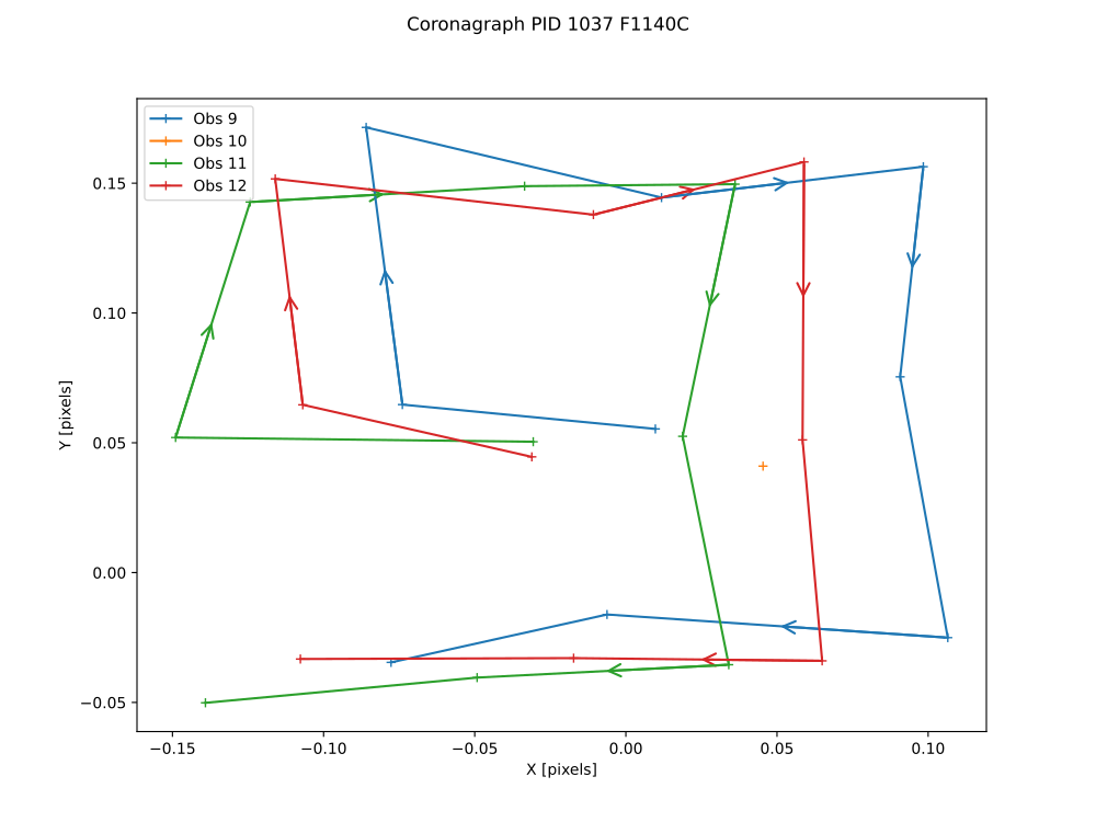
Exemple of the plot.compare_dithers() function (not representative of the source code example, but gives a better idea of a real example).
histogram
Quickly display an histogram for an input dataset, using optimised number of bins
import miritools
import numpy as np

data = np.random.normal(size=10000)

fig = miritools.plot.histogram(data, xlabel="Random gaussian")
# fig2 = histogram(data, xlabel="My data", title="My title")
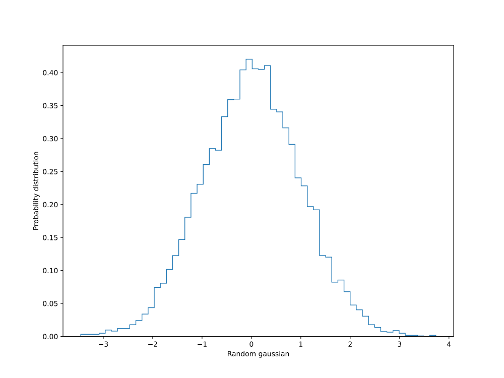
Exemple of the imager.plot.histogram() function
single_image
plot one image with ZScale
import miritools
import numpy as np

image = np.random.random(size=(50, 50))

fig = miritools.plot.single_image(image, vlabel="Flux [mJy]", title="My plot")
fig.savefig("single_image.svg")
Optional parameter:
force_positive: If True, will exclude negative values when computing the Zscale
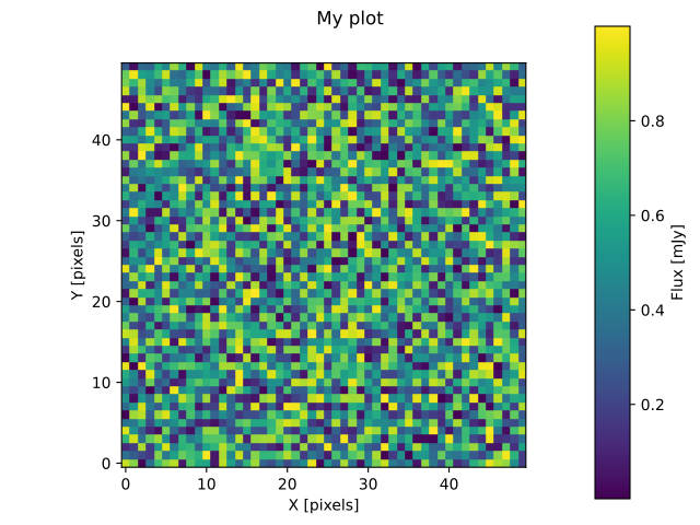
Exemple of the imager.plot.single_image() function
MIRI_flag_images
Expect list (or one) filenames for a level 2 MIRI imager FITS file, will display the flag image for each file. (e.g. saturation is the flag DQ=2 ; Combined flags also work e.g. 7=4+2+1). The title can be constructed from a header keyword (using the title_keyword parameter), or be provided as a list (using the titles parameter, that expect one title per file)
fig = MIRI_flag_images(filenames, flag=2, title_keyword="NGROUPS")
fig2 = MIRI_flag_images(filenames, flag=2, titles=["file1", "file2"])
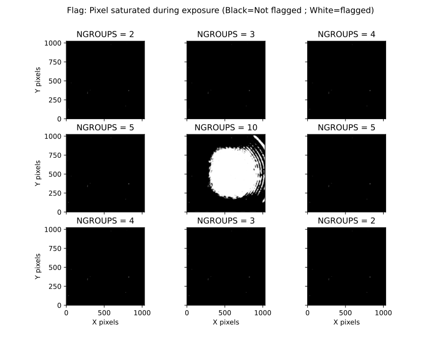
Exemple of the imager.plot.MIRI_flag_images() function
MIRI_saturation_frame
Given one integration ramp image, return the frame number at which each pixel saturate (as an image).
Default is:
figure is not saved to file but you can if you define the filename keyword
frame_to_plot is the last one (for the left image used as a reference)
sat_limit=62000 (at what point the pixel is considered saturated)
# Normal use
fig = miritools.plot.MIRI_saturation_frame(ramp_image, filename="saturation.svg")
Mandatory parameters:
ramp_image as a numpy 3D cube (frame, y, x). Only one integration is accepted, but a cube with an extra 4-th dimension of only one value (1, frame, y, x) will also work.
Optional:
frame_to_plot: Frame used in reference image (left). By default it’s the last one
sat_limit: DN count at which the pixel is considered saturated. By default 62000
filename: If given, will save the figure to a file.
Note
That you can do that later since the figure is returned by the function.
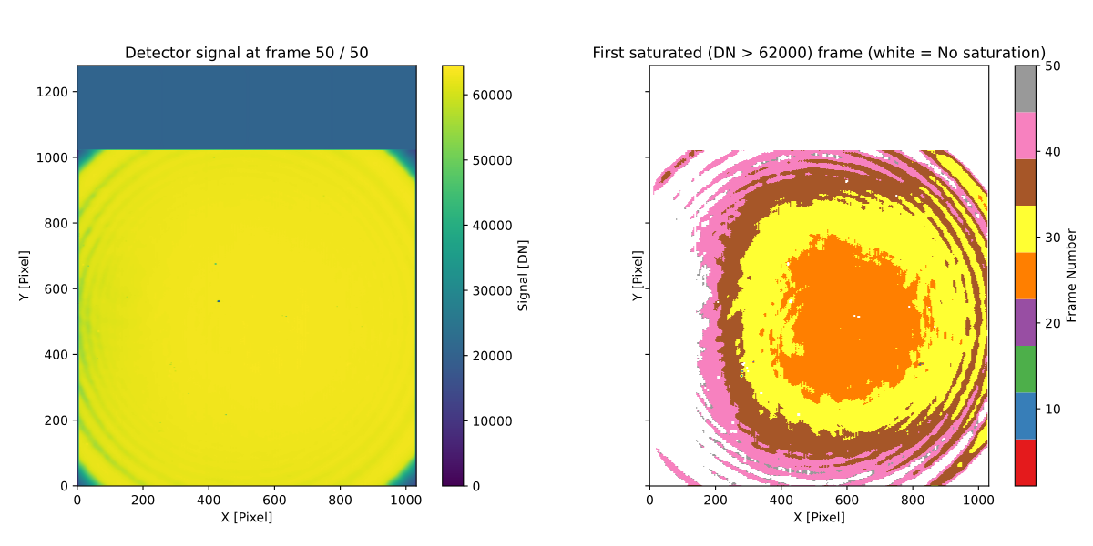
Exemple of the imager.plot.MIRI_saturation_frame() function
MIRI_ramp_flag
This function need a ramp image. The subtelty is that you can’t use the _uncal format that doesn’t have any flag information in it. You have to you the _ramp image that is not saved by default but you can save it manually by reprocessing your data through level 1 with the correct options.
filename = "jw0xxxx006001_03101_00001-seg000_mirimage_ramp.fits"
miritools.plot.MIRI_ramp_flag(filename, flag=4)
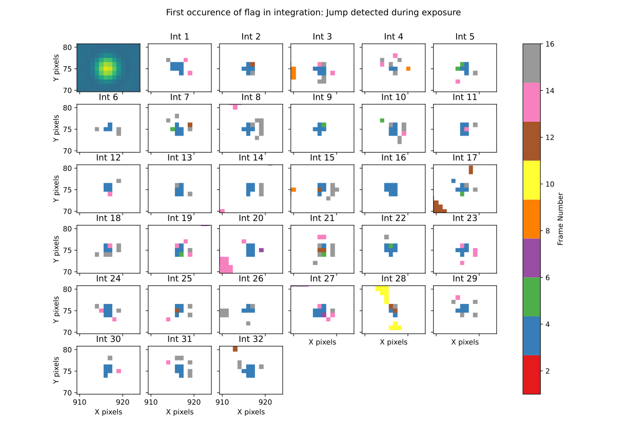
Exemple of the plot.MIRI_ramp_flag() function
pixel_ramps
Will display all integrations from a pixel in a single level 1b exposure.
fig = miritools.plot.pixel_ramps(ramp_image=data, metadata=header, pixel=(639, 367),
                            filename="all_ramps.svg", substract_first=True)
Exemple of the plot.pixel_ramps() function
flag_identifier
Introduced in miritools v3.18.0
Will display all individual flag mask of a single exposure (rate or cal) to identify quickly which flag is causing one specific region to be masked.
Another plot is created, for convenience, with a little explanation for each of the individual flag so you don’t have to look for it
filename = 'jw01052001001_02105_00001_mirimage_rate.fits'

fig = miritools.plot.MIRI_flag_identifier(filename)
plt.show()

Exemple of the plot.flag_identifier() function

Exemple of the plot.flag_identifier() convenience plot
read
Important
When reading multiple files, the filenames must be ordered from oldest to newest file. See list_ordered_files.
MIRI_ramps
Read multiple MIRI ramps
images, metadatas = read.MIRI_ramps(filenames)
MIRI_exposures
Read multiple MIRI datamodel exposures (_cal, or _rates) (given list of filenames)
time, images, metadatas = read.MIRI_exposures(filenames, exclude_from_mask=[4])
MIRI_rateints
Read multiple MIRI datamodel integrations (_rateints) (given list of filenames)
time, images, metadatas = read.MIRI_rateints(filenames, exclude_from_mask=[4])
MIRI_mask_statistics
Given a FITS filename, return the mask statistic of that file (see mask_statistic)
read.MIRI_mask_statistics(filename)
compare_headers
Read multiple FITS files and compare headers. In a first part, all keywords whose value is identical for all files are displayed. In a second part, all keywords with varying values are displayed as a nice table. Note that a list of excluded keywords from part II exist by default, and you can overwrite it
print(read.compare_headers(filenames))

print(read.compare_headers(filenames, exclude_keywords=["DATE-OBS"]))
An example output:
Common values:
    ACT_ID: 01
    APERNAME: MIRIM_FULL
    BITPIX: 8
    BKGDTARG: False
    CAL_VCS: RELEASE
    CAL_VER: 0.18.3
    CATEGORY: COM
    CCCSTATE: OPEN
    CRDS_CTX: jwst_0672.pmap
    CRDS_VER: 10.3.1
    CROWDFLD: False
    DATAMODE: 1
    DATAMODL: ImageModel
    DATAPROB: False
    DATE-OBS: 2021-03-12
    DETECTOR: MIRIMAGE
    DRPFRMS1: 0
    DRPFRMS3: 0
    DURATION: 13.875

Unique values:
Filename                                            BARTDELT       DVA_DEC        DVA_RA  ENG_QUAL      EXPOSURE    HELIDELT     JWST_DX    JWST_DY    JWST_DZ        JWST_X    JWST_Y    JWST_Z    PATT_NUM    SCTARATE       XOFFSET       YOFFSET
------------------------------------------------  ----------  ------------  ------------  ----------  ----------  ----------  ----------  ---------  ---------  ------------  --------  --------  ----------  ----------  ------------  ------------
679/jw00679001001_02101_00001_mirimage_rate.fits     240.365  -7.02173e-07  -2.27691e-07  OK                   1     239.629  0.00715934  -0.156453  -0.169457  -1.51538e+06   -432472   -324870           1     0        -3.43471e-12  -4.06117e-11
679/jw00679001001_02101_00002_mirimage_rate.fits     240.366  -7.02174e-07  -2.27691e-07  SUSPECT              2     239.63   0.00715934  -0.156453  -0.169457  -1.51538e+06   -432472   -324870           1     0        -3.43471e-12  -4.06117e-11
679/jw00679001001_02101_00003_mirimage_rate.fits     240.367  -7.02149e-07  -2.27694e-07  OK                   3     239.631  0.00715984  -0.156448  -0.169453  -1.51537e+06   -432481   -324880           2     0         0.015057     -7.50022e-05
utils
get_exp_time
For a FITS filename, return the start time of the exposure as a time object
time = get_exp_time(metadata)
reorder_miri_input_folder
(Introduced in v3.10.0)
Given an input folder (relative or absolute path), will search for all .fits file in it, assumed to be JWST MIRI outputs. Will then move them and organize them according to their PID and observation ID. This function is used in CAP104, 202, 501, 502 to ensure the input folder will have the expected structure, no matter how the data is retrieved.
A bash script is automatically created in the input folder cancel_miri_reorder.sh to allow you to revert the folder back to its previous state. This file is automatically overwritten by default. Use the option overwrite=False if you want the function to stop before moving anything, in case this script already exist.
If you want to test the function without moving anything, you can use the parameter dryrun=True.
import miritools

miritools.utils.init_log()

input_folder = "/local/home/ccossou/tmp/MAST_rehearsal_data"

imlib.utils.reorder_miri_input_folder(input_folder, dryrun=True)
# imlib.utils.reorder_miri_input_folder(input_folder)
list_files
Given a pattern (using glob) will retrieve a list of FITS filenames, return an error if no files are found (just a wrapper of glob that check if there are matches)
filenames = list_files("simulations/*_cal.fits")
list_ordered_files
Given a pattern (using glob) will retrieve a list of FITS filenames, then order them from oldest (first) to newest (last)
filenames = list_ordered_files("simulations/*_cal.fits")
filenames = list_ordered_files("simulations/*.fits", jpl=True)
lambda_over_d_to_pixels
Compute λ/d in pixel (valid for JWST MIRI Imager) for the given wavelength in microns
size = lambda_over_d_to_pixels(10)
optimum_nbins
Given a dataset destined to be used in a histogram, will return the apropriated number of bins necessary to view the dataset (assuming you display between min and max of that dataset)
nbins = optimum_nbins(dataset)
fig, ax = plt.subplots()
ax.hist(dataset, bins=nbins, density=True, histtype="step")
timer
Decorator to time how long it takes for a function to run, then display it:
@miritools.utils.timer
def my_func():
    continue
init_log
Init logging package. The example below show how to use the extra_config, but a simple call without argument should be enough in most cases:
extra_config = {"loggers":
        {

            "paramiko":
            {
                    "level": "WARNING",
                },

            "matplotlib":
            {
                    "level": "WARNING",
                },

            "astropy":
            {
                    "level": "WARNING",
                },
        },}

miritools.utils.init_log(log="miritools.log", stdout_loglevel="INFO", file_loglevel="DEBUG", extra_config=extra_config)
write
write_fits
Function to write an image to a FITS file with or without a header
write.write_fits(image, "output.fits", header=header)
write.write_fits(image, "output.fits.gz")
write_jwst_fits
Function to write an image to a FITS file and make it look like a JWST image (i.e header in extension 0 and data in extension 1 called SCI)
write.write_jwst_fits(image, "output.fits", header=header)
write.write__jwst_fits(image, "output.fits.gz")
fits_thumbnail
retrieve data from extension 1 (by default) and write it with the same name as the fits file, with extension .jpg (with ZScale)
write.fits_thumbnail("output.fits")
write.fits_thumbnail("output.fits", fits_extension=0, ext="png")
write.fits_thumbnail("output.fits", fits_extension=0, ext="png")
write_thumbnail
write image to file, with ZScale applied
write.write_thumbnail(image, "output.jpg")